We aim to find the shortest path connecting a start point and an end point on a plane. Both the departure direction at the start point and the arrival direction at the end point are predefined, and there is a constraint on the maximum allowable curvature of the path.
This problem is formulated as a constrained optimization problem, and it has been proven that the shortest path consists of a combination of circular arcs with maximum curvature and straight-line segments. This shortest path is known as the Dubins path. Due to its simplicity in geometric construction, the Dubins path is widely used in motion planning methods for mobile robots, drones, and unmanned underwater vehicles.
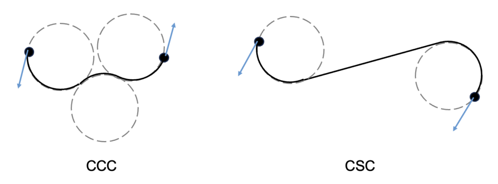
The Dubins path falls into one of two categories: CSC or CCC. Here, C represents a circular arc, and S represents a straight line. The CCC path consists of three consecutive circular arcs that are tangent to each other, while the CSC path consists of one straight line segment and two circular arcs. The radius of the circular arcs is chosen to match the minimum turning radius of the vehicle, which corresponds to the given maximum curvature constraint. Since the CCC path is selected only when the distance between two points is relatively short, we will focus exclusively on the CSC path in this discussion.
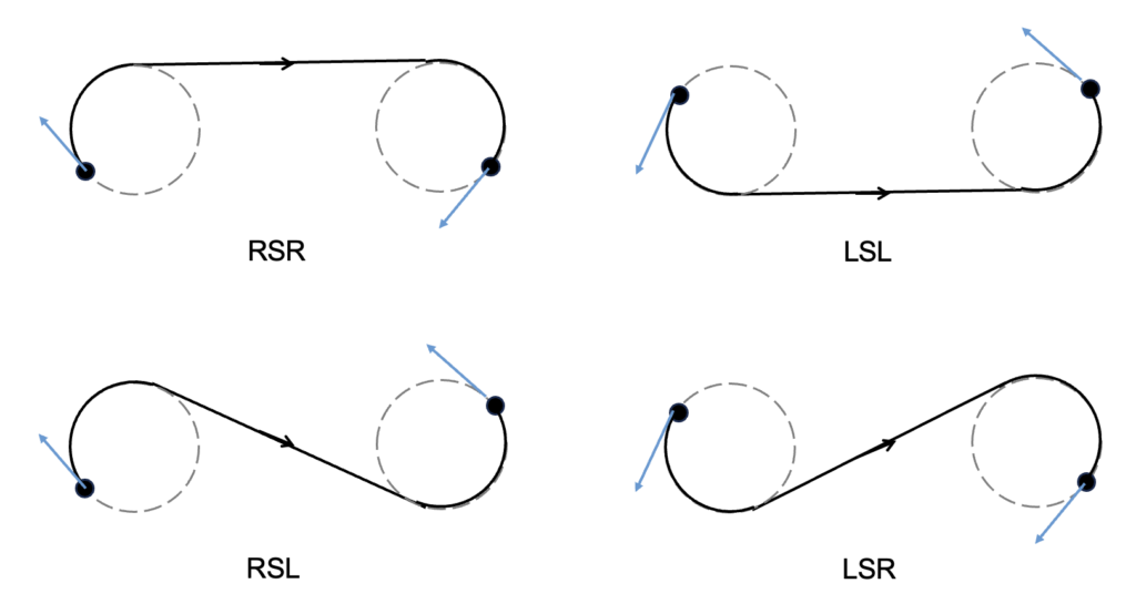
CSC consists of four types: RSR, LSL, RSL, and LSR. Here, R represents a right turn, L represents a left turn, and S represents a straight segment. The shortest path is determined by comparing the distances of these four possible paths.
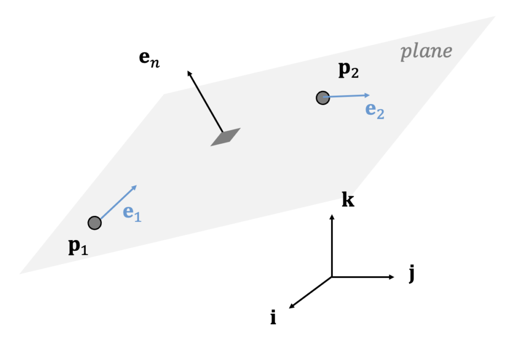
Typically, Dubins paths are designed on the x-y plane. However, in this case, we aim to design the path on an arbitrary plane in 3D space, considering future scalability.
In a plane, the four types of Dubins paths can be designed using the start point \(\mathbf{p}_1\) and end point \(\mathbf{p}_2\), along with a unit vector (or direction vector) \(\mathbf{e}_1\) representing the direction at the start point and another direction vector \(\mathbf{e}_2\) at the end point. However, the vector (\(\mathbf{p}_2-\mathbf{p}_1\)) and the direction vectors \(\mathbf{e}_1\) and \(\mathbf{e}_2\) must all lie on the same plane. In the Figure below, a unit vector perpendicular to the plane is represented as \(\mathbf{e}_n\).
From a given starting point and direction vector, there are two tangent circles on the left and right, as shown in the Figure below. The radius of these circles corresponds to the minimum turning radius (or maximum curvature) \(R\) of the vehicle. The vehicle can travel along these circular arcs by turning either left or right, following the direction of the circle’s curvature. The distinction between left and right is determined based on the vehicle’s direction of motion.
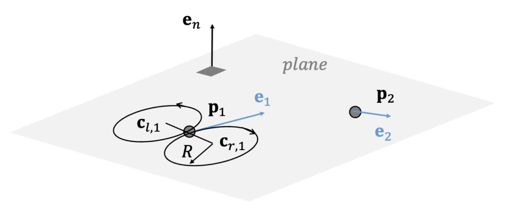
The centers of the two circles can be calculated such that the direction vector at the starting point is tangent to both circles, as shown below.
\[ \begin{align} \mathbf{c}_{l,1} &= \mathbf{p}_1+R \ \mathbf{e}_n \times \mathbf{e}_1 \tag{1} \\ \\ \mathbf{c}_{r,1} &= \mathbf{p}_1-R \ \mathbf{e}_n \times \mathbf{e}_1 \end{align} \]
Here, \(\mathbf{c}_{l,1}\) represents the center of the left circle tangent to the starting point, and \(\mathbf{c}_{r,1}\) represents the center of the right circle tangent to the starting point. Similarly, the centers of the two circles tangent to the end point on the left and right can be calculated using the same method.
\[ \begin{align} \mathbf{c}_{l,2} &= \mathbf{p}_2+R \ \mathbf{e}_n \times \mathbf{e}_2 \tag{2} \\ \\ \mathbf{c}_{r,2} &= \mathbf{p}_2-R \ \mathbf{e}_n \times \mathbf{e}_2 \end{align} \]
The MATLAB code for calculating the centers of the four circles is as follows.
function [left_c1,right_c1,left_c2,right_c2] ...
                        = circle_with_R(p1,p2,e1,e2,R,en)

%    input: two positions p1, p2 (vectors) and directions e1, e2
%          circle radius R, normal vector to plane en
%    output: centers of four circles
%            left_circle at p1, right circle at p1
%            left circle at p2, right circle at p2
%   (c) st.watermelon


% calculate the centers of the left and right circles at p1
% 'left' means 'rotation axis is the same to plane normal vector'
left_c1 = p1 + R * cross(en, e1);
right_c1 = p1 - R * cross(en, e1);

% calculate the centers of the left and right circles at p2
left_c2 = p2 + R * cross(en, e2);
right_c2 = p2 - R * cross(en, e2);

end
The RSR path consists of making a right turn along the right circle from the starting point \(\mathbf{p}_1\), followed by a straight segment, and then another right turn along the right circle at the end point \(\mathbf{p}_2\) to reach the final point. In the Figure below, the pull-out point (\(\mathbf{q}_1\)) marks the transition from the circular arc to the straight segment, while the wheel-over point (\(\mathbf{q}_2\)) indicates the transition from the straight segment back to the circular arc. The straight line connecting these two points is also shown.
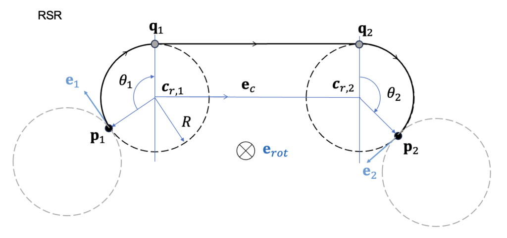
The pull-out point \(\mathbf{q}_1\) and the wheel-over point \(\mathbf{q}_2\) can be calculated as follows.
\[ \begin{align} \mathbf{q}_1 &= \mathbf{c}_1-R \ \mathbf{e}_{rot} \times \mathbf{e}_c \tag{3} \\ \\ \mathbf{q}_2 &= \mathbf{c}_2-R \ \mathbf{e}_{rot} \times \mathbf{e}_c \end{align} \]
where \(\mathbf{e}_{rot}=-\mathbf{e}_n\) represents the direction of rotation of the right circular arc, and \(\mathbf{e}_c\) is the unit vector pointing from the center of the first circle (\(\mathbf{c}_1= \mathbf{c}_{r,1}\)) to the center of the second circle (\(\mathbf{c}_2= \mathbf{c}_{r,2}\)). It is given as follows:
\[ \begin{align} \mathbf{e}_c= \frac{\mathbf{c}_2- \mathbf{c}_1}{‖\mathbf{c}_2- \mathbf{c}_1‖_2} \tag{4} \end{align} \]
The rotation angle \(\theta_1\) for moving from point \(\mathbf{p}_1\) to \(\mathbf{q}_1\) can be calculated as follows.
\[ \begin{align} & \phi_1= \cos^{-1} \left( \frac{(\mathbf{p}_1-\mathbf{c}_1 ) \cdot (\mathbf{q}_1- \mathbf{c}_1 )}{R^2} \right) \tag{5} \\ \\ & \theta_1= \begin{cases} \phi_1, & \mbox{if } \mathbf{e}_1 \cdot \mathbf{e}_{d1} \ge 0 \\ 2\pi- \phi_1, & \mbox{else } \end{cases} \end{align} \]
where \(\mathbf{e}_{d1}\) is the unit vector pointing from \(\mathbf{p}_1\) to \(\mathbf{q}_1\).
\[ \begin{align} \mathbf{e}_{d1}= \frac{ \mathbf{q}_1-\mathbf{p}_1}{‖\mathbf{q}_1-\mathbf{p}_1 ‖_2} \tag{6} \end{align} \]
Similarly, the rotation angle \(\theta_2\) for moving from \(\mathbf{q}_2\) to \(\mathbf{p}_2\) can be calculated as follows.
\[ \begin{align} & \phi_2= \cos^{-1} \left( \frac{(\mathbf{p}_2-\mathbf{c}_2 ) \cdot (\mathbf{q}_2- \mathbf{c}_2 )}{R^2} \right) \tag{7} \\ \\ & \theta_2= \begin{cases} \phi_2, & \mbox{if } \mathbf{e}_2 \cdot \mathbf{e}_{d2} \ge 0 \\ 2\pi- \phi_2, & \mbox{else } \end{cases} \end{align} \]
where \(\mathbf{e}_{d2}\) is the unit vector pointing from \(\mathbf{q}_2\) to \(\mathbf{p}_2\).
\[ \begin{align} \mathbf{e}_{d2}= \frac{ \mathbf{p}_2-\mathbf{q}_2}{‖\mathbf{p}_2-\mathbf{q}_2 ‖_2} \tag{8} \end{align} \]
The LSL path consists of making a left turn along the left circle from the starting point \(\mathbf{p}_1\), followed by a straight segment, and then another left turn along the left circle at the end point \(\mathbf{p}_2\) to reach the final point. In the Figure below, the pull-out point (\(\mathbf{q}_1\)) marks the transition from the circular arc to the straight segment, while the wheel-over point (\(\mathbf{q}_2\)) indicates the transition from the straight segment back to the circular arc. The straight line connecting these two points is also shown.
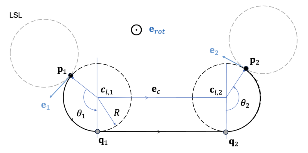
The pull-out point (\(\mathbf{q}_1\)), the wheel-over point (\(\mathbf{q}_2\)), and the rotation angles (\(\theta_1, \ \theta_2\)) can be calculated using the same equations (3)\(\sim\)(8) as the RSR path by applying the following substitutions.
\[ \begin{align} & \mathbf{e}_{rot}= \mathbf{e}_n \tag{9} \\ \\ & \mathbf{c}_1= \mathbf{c}_{l,1} \\ \\ & \mathbf{c}_2= \mathbf{c}_{l,2} \end{align} \]
The distance \(s_f\) between two points \(\mathbf{p}_1\) and \(\mathbf{p}_2\) along the RSR and LSL paths is calculated by summing the lengths of the circular arcs and the straight segment.
\[ \begin{align} s_f=R \theta_1+ ‖ \mathbf{q}_2- \mathbf{q}_1 ‖_2+R \theta_2 \tag{10} \end{align} \]
The MATLAB code for calculating the pull-out point (\(\mathbf{q}_1\)), the wheel-over point (\(\mathbf{q}_2\)), the rotation angles (\(\theta_1, \ \theta_2\)), and the travel distance from the starting point (\(\mathbf{p}_1\)) to the end point (\(\mathbf{p}_2\)) along the RSR and LSL paths is as follows.
% (c) st.watermelon
%
% RSR --------------------------------------------
function param = RSR(right_c1, right_c2, p1, p2, e1, e2, R, en)

c1 = right_c1;
c2 = right_c2;
e_rot = -en;  % right circle rotation axis

[dist, q1, q2, the1, the2] = oneSone(c1, c2, p1, p2, e1, e2, R, e_rot);

param.dist = dist;
param.q1 = q1;
param.q2 = q2;
param.c1 = c1;
param.c2 = c2;
param.the1 = the1;
param.the2 = the2;
param.rot1 = e_rot;
param.rot2 = e_rot;

end


% LSL --------------------------------------------
function param = LSL(left_c1, left_c2, p1, p2, e1, e2, R, en)

c1 = left_c1;
c2 = left_c2;
e_rot = en;  % left circle rotation axis

[dist, q1, q2, the1, the2] = oneSone(c1, c2, p1, p2, e1, e2, R, e_rot);

param.dist = dist;
param.q1 = q1;
param.q2 = q2;
param.c1 = c1;
param.c2 = c2;
param.the1 = the1;
param.the2 = the2;
param.rot1 = e_rot;
param.rot2 = e_rot;

end


% common code in RSR and LSL --------------------------
function [dist, q1, q2, theta1, theta2] = oneSone(c1, c2, p1, p2, e1, e2, R, e_rot)

e_c = (c2-c1)/norm(c2-c1);

q1 = c1 - R*cross(e_rot,e_c);
e_d1 = (q1-p1)/norm(q1-p1);

q2 = c2 - R*cross(e_rot,e_c);
e_d2 = (p2-q2)/norm(p2-q2);

theta1 = acos((p1-c1)'*(q1-c1)/R^2);
if e1'*e_d1 < 0
    theta1 = 2*pi - theta1;
end

theta2 = acos((p2-c2)'*(q2-c2)/R^2);
if e2'*e_d2 < 0
    theta2 = 2*pi - theta2;
end

dist = R*theta1 + norm(q2-q1) + R*theta2;

end